Historical Trends: Raw and Compressed Data Side by Side

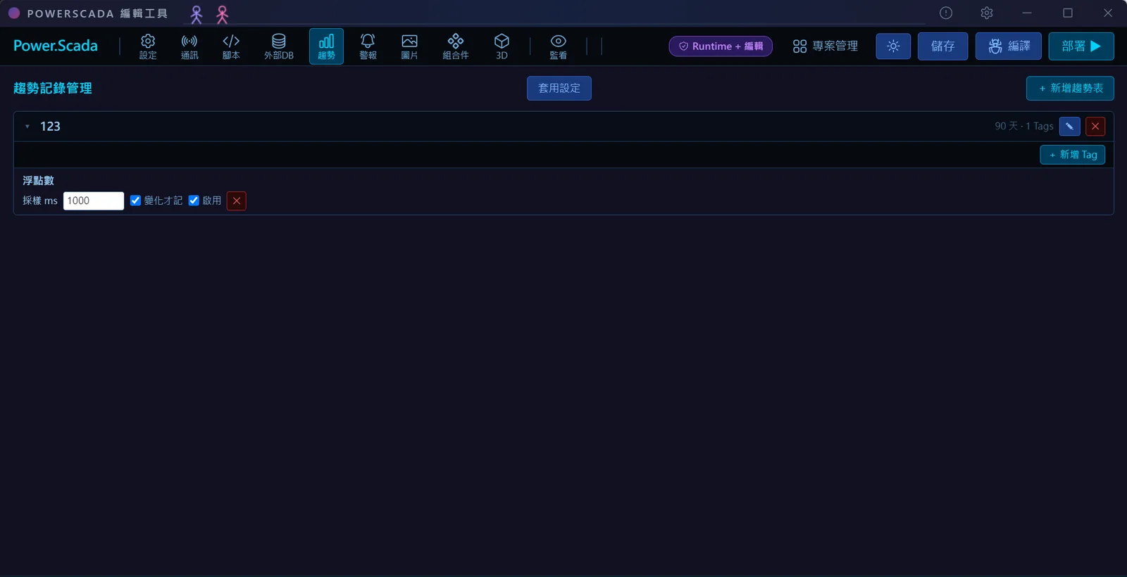
Sampling and retention

The sampling period is shared by the whole table: 1000 ms by default, 100 ms minimum, in 100 ms steps, and we recommend not going below the PLC polling period. Settings take effect within 30 seconds of saving, or immediately with "Apply settings", with no redeployment.

• Each tag can be set to "log on change" and "enabled"; array elements, single bits from bit splitting and built-in system variables can all be logged.
• The compression period defaults to 1 minute, with 15 seconds, 30 seconds, 5 minutes, 15 minutes and 1 hour also available.
• Raw data retention defaults to 90 days (cleaned up daily); compressed data defaults to 730 days, and 0 means forever.
• The header estimates the number of raw and compressed records in real time from the tag count and periods.
• A trend table's tag settings can be exported to and imported from Excel; the "Add tag" bulk picker ticks several tags at once and applies the same settings.

Line trend chart

Each line has a name, color, unit, line width, solid or dashed style, area fill and data points; the Y-axis limits, decimal places, X-axis time format and legend style are adjustable, in flat and industrial styles. The "Independent" layout stacks one row per group vertically, with the current value and limits shown on the left and turning red when out of range.

• Each line takes its data from one of three sources: a live tag, a gateway device variable, or trend history (live points are appended automatically after history loads).
• Interaction: Ctrl + wheel to zoom, drag and two-finger pan, a zoom slider at the bottom and a zoom toolbar (zoom in, zoom out, left, right, back to live); custom start and end queries; 4 Boolean tags for PLC control.
• Automatic downsampling on long ranges: the time each point represents depends on the window length; once it reaches the compression period the chart reads compressed data, draws the average line with a semi-transparent envelope band of the same color for the highs and lows, and the cursor shows average, maximum and minimum.
• The power meter wizard creates a dedicated trend table automatically, which the power meter chart component reads directly.

Export and database

A schedule or a script can export Excel: raw data has one row per instant with every tag in the table on the same row. "Aggregated output" offers 1, 5 or 15 minutes, 1 hour or custom seconds, using average, last, maximum, minimum or maximum and minimum; when the interval is a whole multiple of the compression period it reads compressed data directly, so a one-month report finishes in seconds, and ranges whose raw data has expired can still be exported.

• Trend history can be stored in PostgreSQL, local SQLite (one file per trend table) or an external database.
• Backup as a zip and upload to restore; in high availability (HA) mode the primary and standby sync automatically.
• The time column always uses the project time zone, shown to the millisecond when the period is under 1 second.

Screenshots

How to set it up

1. 1Click "Trends" in the editor top bar and create a trend table by entering a name in the left column.
2. 2In the header, set the sampling period, raw data retention days, compression period and compressed data retention days.
3. 3Click "Add tag" and tick the tags to log (arrays and bits can be expanded), set "log on change" and "enabled", or import from Excel.
4. 4Click "Apply settings" so the logger picks it up immediately.
5. 5Place a line trend chart on the screen, set each line's source to "Trend history" with the trend table and tag, and set the query range, Y-axis, style and layout.
6. 6After deployment, view with the wheel, drag, the toolbar or PLC tags; for long-term reports, create an export task under "Schedules" and tick aggregated output.